Inferring parameters of SDEs using a Euler-Maruyama scheme

This notebook is derived from a presentation prepared for the Theoretical Neuroscience Group, Institute of Systems Neuroscience at Aix-Marseile University.

import warnings

import arviz as az
import matplotlib.pyplot as plt
import numpy as np
import pymc as pm
import pytensor.tensor as pt
import scipy as sp

# Ignore UserWarnings
warnings.filterwarnings("ignore", category=UserWarning)

RANDOM_SEED = 8927
np.random.seed(RANDOM_SEED)

%config InlineBackend.figure_format = 'retina'
az.style.use("arviz-darkgrid")

Example Model

Here’s a scalar linear SDE in symbolic form

\( dX_t = \lambda X_t + \sigma^2 dW_t \)

discretized with the Euler-Maruyama scheme.

We can simulate data from this process and then attempt to recover the parameters.

# parameters
lam = -0.78
s2 = 5e-3
N = 200
dt = 1e-1

# time series
x = 0.1
x_t = []

# simulate
for i in range(N):
    x += dt * lam * x + np.sqrt(dt) * s2 * np.random.randn()
    x_t.append(x)

x_t = np.array(x_t)

# z_t noisy observation
z_t = x_t + np.random.randn(x_t.size) * 5e-3

fig, (ax1, ax2) = plt.subplots(1, 2, figsize=(10, 3))

ax1.plot(x_t[:30], "k", label="$x(t)$", alpha=0.5)
ax1.plot(z_t[:30], "r", label="$z(t)$", alpha=0.5)
ax1.set_title("Transient")
ax1.legend()

ax2.plot(x_t[30:], "k", label="$x(t)$", alpha=0.5)
ax2.plot(z_t[30:], "r", label="$z(t)$", alpha=0.5)
ax2.set_title("All time")
ax2.legend()

plt.tight_layout()

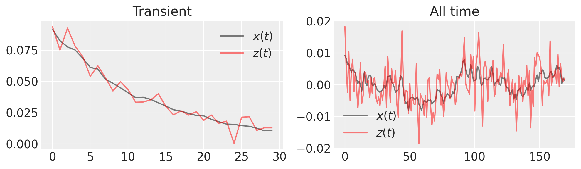
What is the inference we want to make? Since we’ve made a noisy observation of the generated time series, we need to estimate both \(x(t)\) and \(\lambda\).

We need to provide an SDE function that returns the drift and diffusion coefficients.

def lin_sde(x, lam, s2):
    return lam * x, s2

The probability model is comprised of a prior on the drift parameter lam, the diffusion coefficient s, the latent Euler-Maruyama process xh and the likelihood describing the noisy observations zh. We will assume that we know the observation noise.

with pm.Model() as model:
    # uniform prior, but we know it must be negative
    l = pm.HalfCauchy("l", beta=1)
    s = pm.Uniform("s", 0.005, 0.5)

    # "hidden states" following a linear SDE distribution
    # parametrized by time step (det. variable) and lam (random variable)
    xh = pm.EulerMaruyama("xh", dt=dt, sde_fn=lin_sde, sde_pars=(-l, s**2), shape=N, initval=x_t)

    # predicted observation
    zh = pm.Normal("zh", mu=xh, sigma=5e-3, observed=z_t)

Once the model is constructed, we perform inference, which here is via the NUTS algorithm as implemented in nutpie, which will be extremely fast.

with model:
    trace = pm.sample(nuts_sampler="nutpie", random_seed=RANDOM_SEED, target_accept=0.99)

Sampler Progress

Total Chains: 4

Active Chains: 0

Finished Chains: 4

Sampling for now

Estimated Time to Completion: now

Progress	Draws	Divergences	Step Size	Gradients/Draw
	2000	0	0.06	255
	2000	0	0.06	127
	2000	0	0.07	255
	2000	0	0.06	191

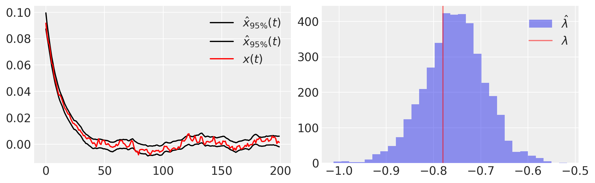
Next, we plot some basic statistics on the samples from the posterior,

plt.figure(figsize=(10, 3))
plt.subplot(121)
plt.plot(
    trace.posterior.quantile((0.025, 0.975), dim=("chain", "draw"))["xh"].values.T,
    "k",
    label=r"$\hat{x}_{95\%}(t)$",
)
plt.plot(x_t, "r", label="$x(t)$")
plt.legend()

plt.subplot(122)
plt.hist(-1 * az.extract(trace.posterior)["l"], 30, label=r"$\hat{\lambda}$", alpha=0.5)
plt.axvline(lam, color="r", label=r"$\lambda$", alpha=0.5)
plt.legend();

A model can fit the data precisely and still be wrong; we need to use posterior predictive checks to assess if, under our fit model, the data our likely.

In other words, we

• assume the model is correct

• simulate new observations

• check that the new observations fit with the original data

# generate trace from posterior
with model:
    pm.sample_posterior_predictive(trace, extend_inferencedata=True)

Sampling: [zh]

plt.figure(figsize=(10, 3))
plt.plot(
    trace.posterior_predictive.quantile((0.025, 0.975), dim=("chain", "draw"))["zh"].values.T,
    "k",
    label=r"$z_{95\% PP}(t)$",
)
plt.plot(z_t, "r", label="$z(t)$")
plt.legend();

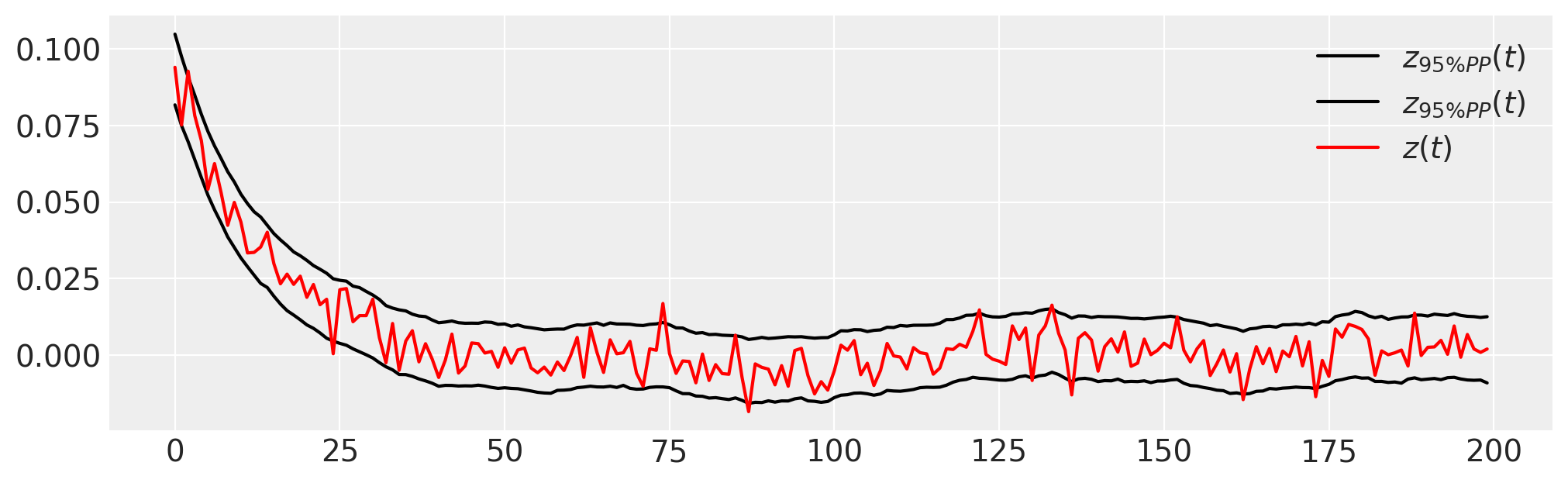
Note that the initial conditions are also estimated, and that most of the observed data \(z(t)\) lies within the 95% interval of the PPC.

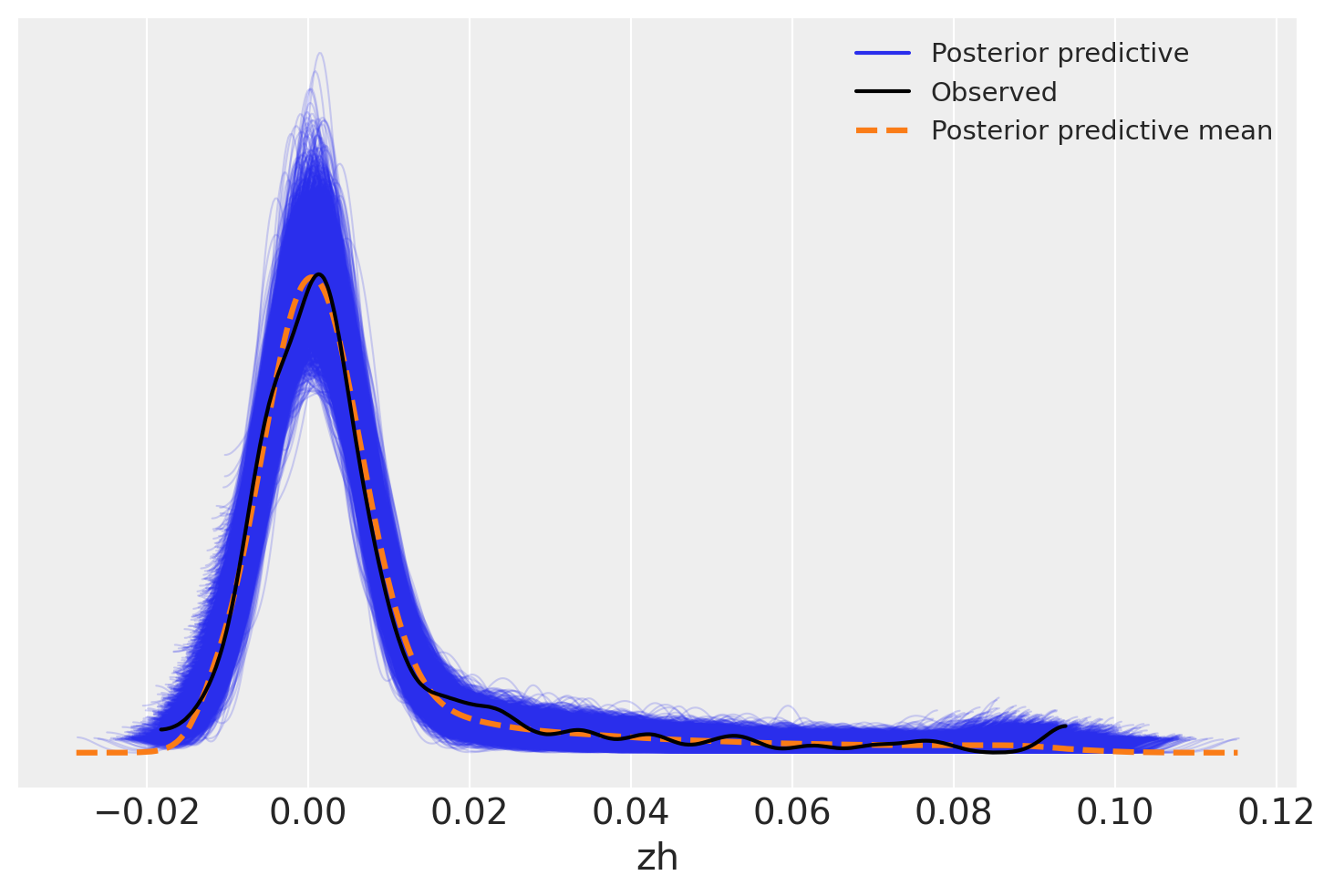
Another approach is to look at draws from the sampling distribution of the data relative to the observed data. This too shows a good fit across the range of observations – the posterior predictive mean almost perfectly tracks the data.

az.plot_ppc(trace)

<Axes: xlabel='zh'>

Authors

• Authored by @maedoc in July 2016

• Updated to PyMC v5 by @fonnesbeck in September 2024

References

%load_ext watermark
%watermark -n -u -v -iv -w

Last updated: Tue Sep 24 2024

Python implementation: CPython
Python version       : 3.12.5
IPython version      : 8.27.0

matplotlib: 3.9.2
pytensor  : 2.25.4
numpy     : 1.26.4
arviz     : 0.19.0
pymc      : 5.16.2
scipy     : 1.14.1

Watermark: 2.4.3